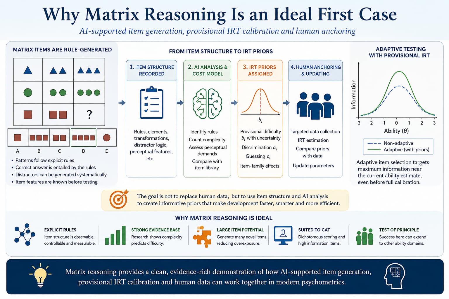
The Case for Matrix Reasoning as a First IRT Demonstration
Matrix-reasoning items provide an unusually tractable setting in which artificial intelligence, explicit item design and Bayesian item response theory can be combined before conventional large-sample calibration is complete.
The known generating structure of a matrix item can be represented as prior information about its likely psychometric parameters. Human responses then update, correct and ultimately anchor those provisional estimates. This proposal requires particular caution when applied to ability testing. A language model may
reproduce what people say about intelligence without reproducing the cognitive processes through which people solve unfamiliar perceptual or spatial problems.
Matrix items are nevertheless a promising first application. This is not because an artificial intelligence can be assumed to respond like a representative human sample. It is because matrix items can be generated from explicit rules whose structural and perceptual properties are observable, controllable and available for statistical modelling.
The AI is therefore not asked to impersonate a population. It assists in constructing, analysing and provisionally locating items whose generating structure is known.
Plain-language summary
This page describes a way of building a new matrix-reasoning test before every item has been fully tested on a large human sample.
Each matrix item is created from known rules. Some items contain one simple change; others require several rules to be discovered and combined. Because the structure of each item is known in advance, it is possible to make a provisional estimate of how difficult the item is likely to be, how well it may distinguish between different levels of ability, and how much guessing may affect the result. These early estimates are not treated as final facts. They are starting assumptions. As people take the test, their responses are used to correct the estimates. The test therefore becomes more accurate as evidence accumulates.
The adaptive part of the system chooses each person’s next item according to what is already known about that person’s responses. It aims to select the item that is expected to provide the most useful new information. A shorter test may therefore achieve a level of precision that would otherwise require many more randomly selected items.
Artificial intelligence assists in generating items, analysing their rule structure, reviewing possible ambiguities and organising the provisional statistical model. It does not replace human calibration. Human responses remain necessary for determining whether the predicted item properties are correct and whether the test is reliable, valid and fair.
The purpose of the demonstration is therefore not to claim that an uncalibrated AI-generated test is already suitable for important decisions. It is to show that explicit item design, provisional statistical estimates, adaptive administration and continuing human calibration can operate together within one coherent system.
Why matrix items are different
A matrix item normally consists of visual elements that change across rows or columns according to one or more rules. These may involve:
- changes of shape, position, number, size, orientation or shading;
- addition, subtraction or combination of elements;
- alternation, progression or distribution;
- several values distributed across a row or column;
- interactions among two or more simultaneous rules.
The correct response is entailed by the generating rules. Distractors can also be generated systematically by embodying incomplete rules, plausible partial solutions, response-elimination shortcuts or common misinterpretations.
This provides more information than is available for an ordinary test item whose difficulty is known only after administration. For a generated matrix item, the developer already knows its formal composition.
the generating structure of a matrix item contains genuine information about its probable psychometric properties, but it does not determine those properties completely.
A unified hierarchical Bayesian IRT model
Let Ypi denote person p‘s response to item i.
Let the three item parameters be ai for discrimination,
bi for difficulty and ci for the lower asymptote.
The complete proposal can be expressed as the following linked generative model. The equations are shown separately because this is more reliable in WordPress and Divi than one large aligned display.
1. Observed response
$$
Y_{pi}\mid\theta_p,a_i,b_i,c_i
\sim
\mathrm{Bernoulli}(\pi_{pi})
$$
2. Three-parameter logistic response probability
$$
\pi_{pi}
=
c_i+
\frac{1-c_i}
{1+\exp\left[-a_i(\theta_p-b_i)\right]}
$$
3. Identification of the ability scale
$$
\theta_p\sim\mathcal{N}(0,1)
$$
4. Structural prior for item difficulty
$$
b_i\mid\mathbf{x}_i,f_i,M
\sim
\mathcal{N}\left(\mu_{b_i},\sigma_{b,i}^{2}\right)
$$
$$
\mu_{b_i}
=
\beta_0+
\mathbf{x}_i^{T}\boldsymbol{\beta}
+
u^{(b)}_{f_i}
$$
5. Structural prior for item discrimination
$$
\log(a_i)\mid\mathbf{z}_i,f_i,M
\sim
\mathcal{N}\left(\mu_{a_i},\sigma_{a,i}^{2}\right)
$$
$$
\mu_{a_i}
=
\alpha_0+
\mathbf{z}_i^{T}\boldsymbol{\alpha}
+
u^{(a)}_{f_i}
$$
6. Prior for the lower asymptote
$$
c_i\mid\mathbf{r}_i,f_i,M
\sim
\mathrm{Beta}\left(\kappa_i m_i,\kappa_i(1-m_i)\right)
$$
$$
\log\left(\frac{m_i}{1-m_i}\right)
=
\log\left(
\frac{1/K_i}{1-1/K_i}
\right)
+
\mathbf{r}_i^{T}\boldsymbol{\delta}
+
u^{(c)}_{f_i}
$$
7. Correlated item-family effects
$$
\mathbf{u}_f
=
\left(
u^{(b)}_f,
u^{(a)}_f,
u^{(c)}_f
\right)^{T}
$$
$$
\mathbf{u}_f
\sim
\mathcal{N}_3\left(\mathbf{0},\mathbf{\Sigma}_u\right)
$$
The multivariate family effect allows related items to share systematic departures from the feature-based predictions. The covariance matrix permits those departures
to be correlated across difficulty, discrimination and guessing.
This formulation brings the whole argument into one model. Responses arise from a conventional three-parameter logistic IRT function, while the item parameters are themselves generated from recorded item characteristics and item-family membership.
Notation
| Symbol | Meaning | Status |
|---|---|---|
| Ypi | Person p‘s scored response to item i | Observed |
| θp | Latent matrix-reasoning ability of person p | Latent |
| ai | Item discrimination | Latent item parameter |
| bi | Item difficulty | Latent item parameter |
| ci | Lower asymptote associated with guessing or partial elimination | Latent item parameter |
| xi | Recorded features used to predict difficulty | Observed design data |
| zi | Recorded features used to predict discrimination | Observed design data |
| ri | Distractor and response-option features used to predict the lower asymptote | Observed design data |
| fi | Item family or generator containing item i | Observed grouping variable |
| Ki | Number of response options for item i | Observed |
| M | The structural model and accumulated design knowledge | Conditioning information |
The response model
The probability that person p answers item i correctly is:
Three-parameter logistic response function
$$
P(Y_{pi}=1\mid\theta_p,a_i,b_i,c_i)
=
c_i+
\frac{1-c_i}
{1+\exp\left[-a_i(\theta_p-b_i)\right]}
$$
The lower asymptote is ci; the curve is centred by bi; and its steepness is governed by ai.
The ability scale must be identified. For an initial calibration population, the convenient convention is:
$$
\theta_p\sim\mathcal{N}(0,1)
$$
This fixes its location and scale. As the bank develops, anchor items and formal linking procedures can maintain comparability across samples and successive calibrations.
Structural prediction of item difficulty
Difficulty is the parameter most directly supported by the known structure of a matrix item. Its conditional prior mean is:
$$
\mu_{b_i}
=
\beta_0+
\mathbf{x}_i^{\mathsf T}\boldsymbol{\beta}
+u^{(b)}_{f_i},
\qquad
b_i\sim N(\mu_{b_i},\sigma_{b,i}^{2}).
$$
The feature vector \(\mathbf{x}_i\) may include:
- the number of independently changing elements;
- the number and type of rules that must be induced;
- whether rules operate across rows, columns or both;
- the number of intermediate results that must be retained;
- interactions among rules;
- perceptual similarity and salience;
- ambiguity in the direction of transformation;
- complexity of the correct response;
- similarity between the key and the distractors;
- availability of response-elimination shortcuts.
The item-specific prior variance \(\sigma_{b,i}^{2}\) expresses how much confidence should be placed in the structural prediction. It can be enlarged when the item contains unfamiliar rule combinations, when expert or AI analyses disagree, or when alternative perceptual organisations appear plausible.
One optional formulation makes that relationship explicit:
$$
\log \sigma_{b,i}
=
\lambda_{b0}
+
\mathbf{q}_i^{\mathsf T}\boldsymbol{\lambda}_b,
$$
The vector \(\mathbf{q}_i\) records sources of uncertainty such as novelty, ambiguity, model disagreement and distance from previously calibrated item families.
The model therefore predicts a distribution of plausible difficulties rather than declaring that a particular structural feature must produce a fixed level of difficulty.
Structural prediction of discrimination
Discrimination is less directly predictable. An item may be difficult because it requires genuine integration of several rules, or because it contains visual confusion unrelated to the intended construct.
Because discrimination must be positive, it is modelled on the logarithmic scale:
$$
\log a_i
\sim
N\!\left(
\alpha_0+
\mathbf{z}_i^{\mathsf T}\boldsymbol{\alpha}
+u^{(a)}_{f_i},
\ \sigma_{a,i}^{2}
\right).
$$
Features supporting higher expected discrimination may include a single defensible solution, identifiable partial-solution distractors, limited dependence on specialist knowledge and a close match between the intended cognitive demand and the target ability range.
Ambiguity, unnecessary visual clutter, accidental cues and dependence on elimination strategies should weaken the prior or increase its variance.
Distractors and the lower asymptote
With \(K_i\) response options, \(1/K_i\) provides a natural starting point for the expected lower asymptote. The hierarchical beta prior in Equation 1 uses:
$$
c_i\sim
\operatorname{Beta}(\kappa_i m_i,\kappa_i(1-m_i)),
\qquad
E(c_i)=m_i,
$$
$$
\operatorname{logit}(m_i)
=
\operatorname{logit}\!\left(\frac{1}{K_i}\right)
+\mathbf{r}_i^{\mathsf T}\boldsymbol{\delta}
+u^{(c)}_{f_i}.
$$
The concentration parameter \(\kappa_i\) controls how tightly the prior is concentrated around \(m_i\). The predictor \(\mathbf{r}_i\) allows the expected asymptote to depart from random guessing when distractors can be eliminated, when one distractor is unusually attractive or when partial rule discovery changes the response probabilities.
For the earliest proof of concept, the simpler and more stable choice \(c_i=1/K_i\) may be used. The hierarchical model describes the natural extension once sufficient
human response data are available.
Item families and correlated departures
Automatically generated items often occur in families sharing the same rule grammar but using different shapes, positions or distractors. Such items should not be assumed to be psychometrically interchangeable.
Equation 1 assigns each family the multivariate effect:
$$
\mathbf{u}_f
=
\left(
u^{(b)}_f,
u^{(a)}_f,
u^{(c)}_f
\right)^{T}
\sim
\mathcal{N}_3\left(
\mathbf{0},
\boldsymbol{\Sigma}_u
\right)
$$
The covariance matrix \(\boldsymbol{\Sigma}_u\) permits, for example, an item family that is systematically harder than predicted also to be more or less discriminating than predicted. This partial pooling stabilises early estimates while retaining item-family differences.
AI as an item-analysis instrument
The proposal does not require synthetic respondents to be treated as human observations. The principal pre-calibration evidence comes from:
- the formal structure used to generate the item;
- cognitive theories of matrix solution;
- previous empirical studies of matrix items;
- expert analysis of perceptual and reasoning demands;
- comparisons with previously calibrated anchor items.
AI can apply this information consistently: identifying rules, counting transformations, comparing alternative interpretations, analysing distractors and locating new items within a library of known structures.
Several models or prompted analyses may also be compared. Their agreement or disagreement contributes to the uncertainty assessment, but their solutions are not human norms.
Human calibration and posterior revision
Let \(D_H\) denote the accumulated human response data, \(\boldsymbol{\Theta}=(\theta_1,\ldots,\theta_P)\) the calibration respondents’ abilities,
\(\boldsymbol{\Phi}=(\boldsymbol{\phi}_1,\ldots,\boldsymbol{\phi}_I)\) the item parameters, and \(\boldsymbol{\Psi}\) the regression coefficients, variance components and other hyperparameters.
The joint posterior is:
$$
p(\boldsymbol{\Theta},\boldsymbol{\Phi},\boldsymbol{\Psi}
\mid D_H,\mathbf{X},\mathbf{Z},\mathbf{R},\mathbf{F},M)
\propto
\left[
\prod_{p=1}^{P}
\prod_{i\in A_p}
p(Y_{pi}\mid\theta_p,\boldsymbol{\phi}_i)
\right]
p(\boldsymbol{\Theta})
p(\boldsymbol{\Phi}\mid
\mathbf{X},\mathbf{Z},\mathbf{R},\mathbf{F},
\boldsymbol{\Psi},M)
p(\boldsymbol{\Psi}).
$$
Structural knowledge supplies the prior model. Human responses supply the likelihood. Posterior inference combines them and records the remaining uncertainty.
The marginal posterior distribution of the item parameters is obtained by integrating over respondent abilities and hyperparameters:
p(\boldsymbol{\Phi}\mid D_H,M)
=
\iint
p(\boldsymbol{\Theta},\boldsymbol{\Phi},\boldsymbol{\Psi}
\mid D_H,M)
\,d\boldsymbol{\Theta}\,d\boldsymbol{\Psi}.
$$
As human evidence accumulates, it increasingly determines the posterior. Large discrepancies between predicted and observed parameters should be retained and investigated because they reveal missing features, ambiguous items, unsuitable distractors, population differences or failures of the structural model.
Posterior predictive checking
Model adequacy can be examined by generating replicated response data:
\widetilde{D}_H
\sim
p(\widetilde{D}_H\mid D_H,M)
=
\iiint
p(\widetilde{D}_H\mid
\boldsymbol{\Theta},
\boldsymbol{\Phi})
p(\boldsymbol{\Theta},
\boldsymbol{\Phi},
\boldsymbol{\Psi}\mid D_H,M)
\,d\boldsymbol{\Theta}\,
d\boldsymbol{\Phi}\,
d\boldsymbol{\Psi}.
$$
Observed and replicated item difficulties, score distributions, residual associations, response-time patterns and family effects can then be compared. Systematic failures indicate where the model should be revised.
Adaptive ability estimation
For a new respondent \(p\), let \(A_p\) be the administered items and \(\mathbf{y}_p=\{y_{pi}:i\in A_p\}\) the observed response pattern.
Initial plug-in approximation
The first demonstration can use posterior means or medians of the item parameters:
$$
p(\theta_p\mid\mathbf{y}_p,\widehat{\boldsymbol{\Phi}})
\propto
p(\theta_p)
\prod_{i\in A_p}
\widehat{\pi}_{pi}(\theta_p)^{y_{pi}}
\left[
1-\widehat{\pi}_{pi}(\theta_p)
\right]^{1-y_{pi}}.
$$
This is the complete Bernoulli likelihood for the respondent’s correct and incorrect responses. It is suitable for a proof of concept, but it treats provisional item estimates as fixed.
Fully Bayesian ability update
A more complete analysis propagates item-calibration uncertainty into the respondent’s score:
$$
p(\theta_p\mid\mathbf{y}_p,D_H,M)
\propto
p(\theta_p)
\int
\prod_{i\in A_p}
\pi_{pi}(\theta_p,\boldsymbol{\phi}_i)^{y_{pi}}
\left[
1-\pi_{pi}(\theta_p,\boldsymbol{\phi}_i)
\right]^{1-y_{pi}}
p(\boldsymbol{\Phi}\mid D_H,M)
\,d\boldsymbol{\Phi}.
$$
Uncertainty about provisional item parameters now contributes directly to uncertainty about the respondent’s ability.
Adaptive item selection as Bayesian experimental design
The next item can be selected by its expected information gain about \(\theta_p\). Let \(\mathcal{C}_p\) denote the eligible items after applying exposure, content and item-family constraints.
$$
i_p^{*}
=
\underset{i\in\mathcal{C}_p}{\operatorname{argmax}}
\;
I\!\left(
\theta_p;Y_{pi}
\mid
\mathbf{y}_p,D_H,M
\right),
$$
$$
I\!\left(
\theta_p;Y_{pi}
\mid
\mathbf{y}_p,D_H,M
\right)
=
\mathbb{E}_{Y_{pi}}
\left[
D_{\mathrm{KL}}
\left(
p(\theta_p\mid\mathbf{y}_p,Y_{pi},D_H,M)
\,\middle\|\,
p(\theta_p\mid\mathbf{y}_p,D_H,M)
\right)
\right].
$$
The selected item is the one expected to reduce uncertainty about the respondent most, averaged across its possible correct and incorrect outcomes.
This is a general Bayesian experimental-design criterion. It includes more than selecting the item whose difficulty is nearest the current ability estimate, and it can account for uncertainty in the item parameters themselves.
Stopping rule
Administration may stop when posterior precision reaches a stated threshold or when a maximum test length is reached:
\sqrt{
\operatorname{Var}
(\theta_p\mid\mathbf{y}_p,D_H,M)
}
\leq \varepsilon
\qquad
\text{or}
\qquad
|A_p|\geq L_{\max}.
$$
Other stopping conditions may be added for minimum content coverage, excessive response time, repeated omissions or insufficient information in the remaining bank.
At the proof-of-concept stage, the resulting score is provisional. The demonstration validates the generation, administration, updating and item-selection architecture; it does not yet justify consequential or norm-referenced interpretations of an individual’s intelligence.
A staged development programme
- Define the rule grammar. Specify permitted transformations, element types, combinations and design constraints.
- Generate a candidate bank. Create original items without reproducing proprietary test material.
- Record item features. Store each item’s rules, perceptual properties, key and distractor rationale.
- Conduct automated and expert review. Reject ambiguity, duplicate solutions, accidental cues and construct-irrelevant demands.
- Assign provisional priors. Estimate distributions for difficulty, discrimination and guessing, including uncertainty.
- Test the adaptive architecture. Examine response collection, scoring, selection, exposure control and stopping.
- Collect targeted human data. Sample respondents and items to test the assumptions most likely to be wrong.
- Update and recalibrate. Compare predictions with observations and revise the structural feature model.
- Validate operational interpretations. Establish reliability, validity, fairness, norms and intended score meanings.
What the proof of concept would establish
A successful demonstration would show that:
- AI-assisted item generation can be connected directly to an IRT item bank;
- known item structure can provide useful provisional parameter information;
- an adaptive test can operate before every item has received conventional large-sample calibration;
- human data can be collected strategically to correct rather than merely initiate the model;
- posterior uncertainty can be reduced progressively as evidence accumulates;
- the same architecture can later be investigated in other ability domains.
It would not establish that AI-generated priors are equivalent to human calibration or that provisional adaptive scores are ready for high-stakes decisions.
Testable predictions
- Structural priors will predict the rank ordering of matrix-item difficulty better than uninformative priors.
- Predictions will improve when rule type, perceptual organisation and distractor structure are included in addition to rule count.
- Difficulty will be more predictable from item structure than discrimination. Items generated from the same formal template will have related but non-identical psychometric
- properties. Large prior-posterior discrepancies will disproportionately identify ambiguity, visual artefacts,
- unmodelled solution shortcuts or population-specific demands.
- Where structural priors are positively associated with eventual human-calibrated parameters, adaptive administration based on those priors will produce lower estimation error or posterior uncertainty than random administration of equal length.
- Adaptive accuracy and precision will improve as human calibration data accumulate and broad structural priors are replaced by empirically anchored posterior distributions.
The complete inferential pathway
\text{Explicit item design}
\longrightarrow
p(\boldsymbol{\Phi}\mid M)
\longrightarrow
p(\boldsymbol{\Phi}\mid D_H,M)
\longrightarrow
p(\theta_p\mid\mathbf{y}_p,D_H,M)
\longrightarrow
\text{continuing posterior revision}.
$$
Conclusion
Matrix reasoning is not an exception to the need for human validation. It is an especially suitable domain in which to investigate whether useful psychometric information exists before conventional calibration begins.
The formal rules of item generation provide evidence about likely cognitive demand. Artificial intelligence can help extract, organise and apply that evidence. Hierarchical Bayesian IRT can represent it as a provisional probability model rather than an established fact. Carefully selected human responses can then correct the predictions and anchor the resulting scale.
The central empirical question is:
Selected evidence
Freund, Hofer and Holling, Explaining and Controlling for the Psychometric Properties of Computer-Generated Figural Matrix Items. Automatically generated matrix items demonstrated Rasch fit, with item difficulty reasonably explained by the implemented task parameters.
Blum and Holling, Automatic Generation of Figural Analogies with the IMak Package. Rule count was associated with lower accuracy and longer response times, while explanatory rule models accounted for a substantial proportion of item-difficulty variance.
Zorowitz, Chierchia, Blakemore and Daw, An Item Response Theory Analysis of the Matrix Reasoning Item Bank. Complexity robustly predicted difficulty in a large adult sample, although nominal item clones could not be assumed to be psychometrically exchangeable.